01Quantitative questioning as a source of information
An analyst’s question can connect reported results with the assumptions behind an investment view. ECQDI examines the quantitative character of those questions.
External analysts bring company knowledge, sector expertise and financial models to the call. A question about an operating measure, a forecast assumption or the relationship between reported figures may reflect work completed before the conversation begins. These contributions provide an observable record of the issues that informed participants choose to examine.
The research rationale is that this record may contain information beyond historical prices and trading volumes. Quantitative questioning could indicate close scrutiny of a company’s operating outlook or an effort to resolve uncertainty in an existing model. It can also accompany concern, disagreement or unusually complex reporting. The interpretation therefore needs to be tested against subsequent outcomes.
Related research supports examining analyst contributions. Mayew, Sharp and Venkatachalam find that participating analysts issue more accurate and timely forecasts immediately after calls than nonparticipants [1]. Rennekamp, Sethuraman and Steenhoven study conversational engagement between managers and analysts as an informative characteristic of the interaction [2]. These findings motivate attention to questioning and conversation; they do not establish the return contribution of ECQDI.
Quantitative dynamics and intensity describes the factor’s perspective. Intensity concerns the quantitative character of external analyst contributions. Dynamics concerns how successive observations differ within an evolving historical reference. The current score is a deterministic call measurement expressed relative to earlier sector peers. It does not separately estimate sentiment, research quality or the speed of change between calls.
02Data, universe and timing
The analysis joins structured call transcripts, frozen model forecasts and adjusted equity prices. The source archive and the investable research panel serve different roles.
The ECQDI source snapshot contains 78,851 calls from 3,722 tickers. It supports the text measurement and historical sector comparisons. Portfolio tests use the smaller US universe with eligible Qlib forecasts and the required prices. Table 1 distinguishes these inputs from the weekly portfolio sample; a call count is not a count of independent investment tests.
An internal replay reproduces all 48,701 stored version-2 scores. For the portfolio study, the historical reference excludes every call on the observation’s own date, leaving 48,689 eligible scored calls. This stricter ordering removes dependence on the processing order of calls held on the same day. The replay and timing checks are documented in Appendix A.1.
| Input | Coverage | Role in the study |
|---|---|---|
| Call archive | 78,851 calls · 3,722 tickers | Structured transcripts supply external analyst contributions and the historical sector reference. This archive extends beyond the model-eligible portfolio universe. |
| Call scores | 48,701 replayed; 48,689 strict-date | The first count reproduces stored version-2 observations. The second applies the portfolio rule excluding all same-day calls from each historical reference. |
| Model forecasts | 2,259,772 rows · 544 tickers | Frozen stock-ranking predictions across dates and four model seeds. Both arms use the same forecasts; ECQDI is not a model-training feature. |
| Adjusted prices | 782,434 rows · 560 tickers | Frozen adjusted USD prices supply opening trade prices and closing valuations. The same series supports both portfolio arms throughout the study. |
| Score availability | 90.41% of forecast rows | Forecast rows with an eligible prior-call score within the 90-calendar-day limit. Repeated seed rows are included; this is not coverage of all US equities. |
| Weekly formations | 245 starting dates | Portfolio start dates from 10 Jan 2022 to 14 Sept 2026. Only completed holding periods enter the three-, six- and twelve-month return comparisons. |
| Price cut-off | 18 Sept 2026 | Last price session in the frozen evaluation. It determines which horizons have matured and the end date for each continuously invested account. |
The eligible US equity universe
The model panel uses S&P 500 membership snapshots as its reference and applies the baseline’s data requirements. Across the forecast history, it contains 544 distinct tickers; membership and eligibility vary by date. Both arms draw from the same model-eligible US equity universe. Historical membership, delisted stocks and adjusted-price coverage remain part of the data-verification work described in Section 8.
At the call date, score eligibility requires at least $5 million in median daily dollar volume across the latest 60 earlier stock bars, with at least 30 positive observations. The sector reference includes calls with a usable measurement even if their issuer does not meet that trading-liquidity condition. The condition governs whether a score is supplied for the issuer; it does not reduce the historical reference to the same investable stocks.
From call date to portfolio decision
- Call observation
- Measure external questioning against calls from strictly earlier dates in the same sector.
- Next session open
- The call score first becomes eligible at the next US trading session’s opening.
- Weekly decision
- Join the eligible score to the preceding close’s model prediction at the scheduled decision.
A Friday call can enter Monday’s selection if Monday is a trading day. A Tuesday call becomes eligible on Wednesday, while the weekly strategy normally waits until its next scheduled decision. US market sessions determine the execution date. A new call therefore does not automatically produce an immediate trade.
Information timing. The source’s same-day transcript delivery leaves a buffer before the next-session execution used here. The historical study applies that date convention to stored transcript versions. Verification of later revisions is separate from checking call dates; prospective evaluation should retain the score and publication time actually available when the decision was made.
03From a call to ECQDI
ECQDI expresses a call’s quantitative questioning relative to its sector history, in a form that can be joined to an equity panel by date and ticker.
- Observe: Identify external analysts’ contributions in the structured question-and-answer record.
- Measure: Apply the same deterministic text measurement to each eligible call.
- Contextualize: Compare the observation with earlier calls in its historical sector reference.
- Evaluate: Apply the supplied score to a fixed selection rule and compare matched portfolios.
The measurement uses external analyst contributions. Management’s prepared remarks and answers are excluded. Fixed extraction rules make the calculation repeatable without fitting a language model, retraining predictive text weights or assigning a sentiment label to each new call.
The reference covers the preceding 365 calendar days and requires at least eight usable calls in the same sector. A score of 0.80 means that 80% of those reference observations have a strictly lower measurement. Equal measurements are not counted as lower. This expresses the call’s relative position; it is neither an 80% probability of a price rise nor a forecast of the company’s earnings.
- Field:
ecqdi_score, a supplied value between 0 and 1. - Direction: Higher values indicate greater relative quantitative intensity.
- Persistence: A call’s score is carried forward unchanged while it remains eligible.
- Expiry: The study accepts call ages of 1-90 calendar days at the decision date.
- Missing score: No eligible value for that stock and date; zero remains a valid score.
Daily availability and expiry
The date in the daily sample identifies the decision session for which the supplied value is eligible. Its underlying call can be older: a call from three weeks earlier may still support today’s value. ECQDI retains the sector context from the call date. It does not re-rank that same call every morning as other companies report.
The portfolio uses the latest eligible scored call before its decision date. A newer scored call replaces it. A later call that has no eligible score does not itself replace the earlier scored observation. The prior value remains usable only through day 90 after its own call date; day 91 is outside the study’s freshness window. Carrying the value into another daily row does not reset its age.
Use the value supplied for the decision date. The score CSV already applies the call-date ordering and expiry rules, so an additional day of delay is unnecessary. A blank should remain missing. In buy & hold, subsequent score expiry alone does not trigger a sale; weekly rebalancing uses the eligible observations at each new decision.
What a missing score means
- No earlier scored call: No eligible scored observation precedes the decision date.
- Unusable input: The call lacks the required analyst text or sector information.
- Insufficient peers: Fewer than eight usable sector calls are available in the reference window.
- Liquidity eligibility: Earlier price observations are insufficient or the liquidity floor is unmet.
- Expired observation: The latest eligible scored call is more than 90 calendar days old.
These conditions explain why a current value may be unavailable. An ineligible new call can coexist with an older, still-valid score. The primary portfolio keeps stocks with missing values eligible under the model ranking and gives them no score penalty. The scored-only control removes them from both arms before selection. Missingness is an eligibility state, not a positive or negative investment view.
Scope of disclosure. This note documents the rationale, inputs, reference window, timing and portfolio application. The exact extraction rules, normalization and raw measurement remain proprietary. The supplied score and the rule in Section 4.2 allow researchers to test its usefulness without reconstructing the text-measurement engine.
04The paired portfolio design
Every comparison begins with the same model forecasts. ECQDI changes selection priority; capital, execution and accounting remain shared.
4.1 Baseline model and training chronology
The baseline combines Microsoft’s Qlib research framework [3], 157 available price and volume features from the Alpha158 family [4], and LightGBM, a gradient-boosted decision-tree model [5]. It learns relationships between historical market features and later returns, then ranks eligible stocks. The training target is the adjusted return from the next session’s open to the 42nd session’s close, standardized across stocks on each training date.
Annual expanding windows admit only training returns that have ended before the test year. Models use 200 boosting rounds and four fixed seeds: 19, 41, 73 and 101. These identify different randomized training runs on the same market history. All 20 year/seed training records satisfy the recorded date-ordering checks. Both arms reuse the frozen forecasts; the baseline is not retrained with ECQDI.
Role of the published software. Qlib and LightGBM provide the modelling foundation. Our US data preparation and weekly simulator are custom implementations, rather than an unchanged official Qlib benchmark. Their authors have not validated or endorsed ECQDI.
4.2 Which score changes the selection?
The factor input is the eligible daily ecqdi_score. The model prediction ranks investment candidates, while ECQDI adjusts their selection priority. The primary study gives lower priority to the lowest 20% of available scores across the eligible stock universe at each decision.
- Use the decision-date score. Join by ticker and date to the same prior-close forecasts for both arms. For a call-level history, use the latest eligible scored call from an earlier date, at most 90 calendar days old. The daily CSV has already applied these rules.
- Rank available scores before selecting holdings. Sort all available scores from low to high and divide each average ordinal rank by the number of scored candidates, N. Ties receive their average rank. Deprioritize percentiles at or below 0.20 when N is at least 30; otherwise retain the model ranking. Missing scores do not enter this calculation and receive no penalty.
- Select 50 stocks deterministically. The baseline sorts forecasts from highest to lowest, breaking ties alphabetically by ticker. The factor arm places unpenalized candidates first, then penalized candidates, with the same model and ticker order within each group. Take the first 50. Penalized stocks can fill remaining places; fewer than 50 eligible candidates prevent a portfolio from being formed.
- Apply the rule at the scheduled decision. Buy & hold selects once at entry. Weekly rebalance repeats the rule using the current eligible scores and forecasts, and resets target weights under the shared account assumptions.
Example. With 100 scored candidates and no ties, score ranks 1-20 receive lower priority. The raw score at the boundary changes with the date and universe. A score of 0.20 is therefore not a universal sell threshold, and a high score alone does not secure a place among the 50 holdings.
- Baseline: Select the 50 highest-ranked eligible stocks from the frozen model forecasts.
- With ECQDI: Adjust selection priority using the score, then select 50 stocks.
Two rankings have different roles. The ECQDI value locates the call within its earlier sector history. The portfolio rule then ranks those supplied values across today’s eligible candidates. Model predictions determine the order within each priority group. This tests ECQDI as an addition to the existing selection process, rather than as a standalone portfolio ranking.
4.3 Capital, execution and valuation
- Formation: A new pair starts at the first eligible US trading session of each week, normally Monday. Each account begins with $1 million and is evaluated separately from earlier formations.
- Allocation: Fifty positions share 95% of pre-trade equity equally. Fractional adjusted share units are allowed; fees reduce the residual cash balance, and cash earns no interest.
- Buy & hold: Keep the initial share quantities through the evaluation horizon. There is no scheduled rebalancing, and a later score change or expiry alone does not cause a trade.
- Weekly rebalance: Reapply selection and equal target weights at the first session of each week. This includes resizing retained positions, with costs charged on their executed trade amounts.
- Trading costs: Charge 10 bp, or 0.10%, of every executed buy and sell notional. The primary comparison does not separately model spreads, market impact or trading capacity.
- Prices: Execute at frozen adjusted opens and value holdings at adjusted closes plus cash. Corporate actions are represented in the price series; no additional dividend cash flow is added.
- Evaluation: Use 3, 6 and 12 calendar months, marked at the last session close on or before the anniversary. Remaining holdings are not liquidated, so there is no terminal sale fee.
4.4 Measuring the contribution and its uncertainty
For each formation, seed and horizon, subtract the baseline return from the ECQDI return. Average the four seed differences within the formation, then give every completed formation equal weight. A positive difference means the factor portfolio earned more after the stated costs. The result is a holding-period return difference, without annualization or adjustment for other equity-factor exposures.
Weekly portfolios share much of their holding period. To reflect that dependence, we repeatedly draw contiguous blocks of weekly differences and recompute the mean, wrapping from the end of the series to its beginning when necessary [6]. The spread of those recomputed means provides the reported uncertainty interval.
- Resamples: Recompute the average on 5,000 block-based redraws of the same weekly history.
- Block lengths: Use 13, 26 and 52 weeks for the 3-, 6- and 12-month comparisons.
- Reported interval: The 2.5th to 97.5th percentiles of the resampled mean differences.
An interval spanning zero permits both no improvement and a positive contribution under this procedure. These are estimates for the specified historical comparison. They do not account for every model or threshold explored during the wider research process.
05What the factor added
Buy & hold improves on average at all three horizons. Weekly rebalancing produces a smaller and less consistent contribution.
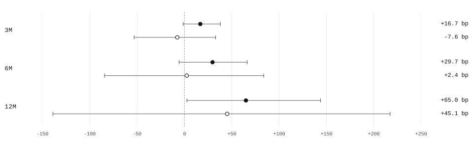
The points show the average return difference; the horizontal lines show its uncertainty interval. At six months, buy & hold adds +29.7 bp with a range from -5.7 to +66.3 bp. At twelve months, the mean is +65.0 bp and the range is +2.6 to +143.8 bp. The latter is the only primary interval entirely above zero.
| Horizon | Baseline | With ECQDI | Difference | 95% interval, bp | Formations |
|---|---|---|---|---|---|
| Buy & hold | |||||
| 3M | 3.22% | 3.39% | +16.7 bp | [-1.4, +37.9] | 232 |
| 6M | 6.05% | 6.34% | +29.7 bp | [-5.7, +66.3] | 219 |
| 12M | 14.53% | 15.18% | +65.0 bp | [+2.6, +143.8] | 193 |
| Weekly rebalance | |||||
| 3M | 2.46% | 2.39% | -7.6 bp | [-53.2, +32.9] | 232 |
| 6M | 5.34% | 5.36% | +2.4 bp | [-84.5, +83.8] | 219 |
| 12M | 11.39% | 11.85% | +45.1 bp | [-139.0, +217.4] | 193 |
In the six-month buy & hold comparison, mean returns are 6.05% for the model baseline and 6.34% with ECQDI. The overlay changes an average of 8.8 of the 50 entry holdings across all weekly formations. Its measured contribution comes from adjusting a model-ranked portfolio; the table does not describe the return of buying every high-scoring stock.
The three horizons include 232, 219 and 193 completed formations respectively. A longer horizon requires more subsequent prices, so its set of starting dates is smaller. Recent incomplete accounts are excluded from the horizon averages. The four seeds are averaged within each formation and share the same underlying market history.
Selection at entry and repeated rebalancing answer different questions
Buy & hold asks whether the initial choice of stocks improves the later account value. Weekly rebalancing also reflects new selections, changing target weights and repeated trading. A useful entry observation need not improve every subsequent rebalance. The near-zero six-month weekly contribution and the weaker continuous accounts make this distinction central to interpreting ECQDI.
06Testing the assumptions
We change costs, selection strength and stock coverage while keeping the model forecasts fixed. These checks identify which implementation choices affect the result.
6.1 What changes when trading costs or frequency change?
The follow-up applies 0, 10 and 25 bp to every executed buy or sell. Both arms are recomputed at each rate. For buy & hold, the opening trade amount is the same in both arms, so higher costs reduce their returns equally and leave the six-month difference near +30 bp.
Repeated trading has a larger effect on continuously invested accounts. At 10 bp, weekly rebalancing produces mean CAGR of 7.24% for the baseline and 6.90% with ECQDI. The factor’s shortfall remains when fees are removed. Trading costs therefore do not fully explain the weaker weekly result.
Monthly rebalancing changes the outcome: at 10 bp, mean CAGR is 6.82% for the baseline and 6.95% with ECQDI, with two of the four seeds improving. Here the account trades at entry and then at the first session of each subsequent calendar month. The small gain makes slower implementation worth examining, but does not establish an optimal trading schedule.
View trading-frequency and cost comparisons
| Cost per side | Baseline CAGR | ECQDI CAGR | Difference, pp/year |
|---|---|---|---|
| Weekly rebalance | |||
| 0 bp | 13.89% | 13.37% | -0.51 |
| 10 bp | 7.24% | 6.90% | -0.35 |
| 25 bp | -2.03% | -2.16% | -0.13 |
| Monthly rebalance | |||
| 0 bp | 8.85% | 8.96% | +0.11 |
| 10 bp | 6.82% | 6.95% | +0.13 |
| 25 bp | 3.83% | 4.00% | +0.17 |
Each number is the mean CAGR of four separate continuous accounts. Fixed fees do not measure stock-specific spreads, order-size effects or available trading capacity.
6.2 Does a stronger score rule help?
Giving lower priority to the weakest 10%, 20%, 30% or 50% of scores produces six-month buy & hold differences of +9.2, +29.7, +3.4 and +26.3 bp. The progression is not steadily increasing. All four intervals include zero, and all four rules reduce mean continuous weekly CAGR at the primary cost assumption.
The later 2024-2026 formations have negative six-month buy & hold differences at the 30% and 50% settings. More influence for the score therefore does not consistently improve selection in this study. Section 10 plots the threshold results and sets out how to test a small set of configurations prospectively.
6.3 Does stock coverage or sector allocation explain the result?
- Only stocks with scores: Remove unscored candidates from both arms. The six-month buy & hold difference remains positive at +33.3 bp, while the continuous weekly comparison remains weaker than its own baseline.
- Match sector allocation: Preserve the baseline’s stock count in every sector when selecting the factor portfolio. Six-month buy & hold adds +34.6 bp, with a 95% interval of +1.4 to +70.4 bp.
- Inspect concentration: The largest positive stock contribution is approximately 6.0 bp. Subtracting the five largest positive contributions leaves +12.6 bp of the original +29.7 bp mean difference.
The scored-only comparison changes the universe for both portfolios. Its baseline continuous CAGR rises to 8.68%, and adding ECQDI within that restricted universe lowers it to 8.37%. The higher baseline return belongs to the eligibility screen, rather than to the score’s ordering. Sector matching limits one source of exposure differences, while size, momentum and liquidity need further controls.
View selection and coverage results with uncertainty intervals
| Selection rule | 6M B&H, bp | 95% interval, bp | Weekly CAGR change, pp/year | Seeds improved |
|---|---|---|---|---|
| Lowest 10% | +9.2 | [-15.3, +39.4] | -0.35 | 1/4 |
| Lowest 20% · reference | +29.7 | [-5.7, +66.3] | -0.35 | 1/4 |
| Lowest 30% | +3.4 | [-35.6, +39.4] | -0.95 | 1/4 |
| Lowest 50% | +26.3 | [-30.8, +69.0] | -1.60 | 0/4 |
| Scored-only · 20% | +33.3 | [-1.3, +71.9] | -0.31 | 1/4 |
| Sector-matched · 20% | +34.6 | [+1.4, +70.4] | -0.79 | 0/4 |
The six-month column measures completed buy & hold cohorts. The annualized column measures continuous weekly accounts. These are separate performance measures, each compared with its own matched baseline.
The concentration calculation uses the realized stock contributions after the outcome is known. It is an attribution check, not a portfolio that could have excluded those winners in advance. All checks in this section reuse the same studied period.
07Continuously invested accounts
Overlapping portfolio cohorts describe repeated entry decisions. A continuously invested account follows the experience of carrying the same capital through time.
For each seed and arm, one account starts on 10 January 2022 and is rebalanced weekly through 18 September 2026. The primary allocation and 10 bp trading costs apply throughout. No fresh capital is introduced at later formation dates.
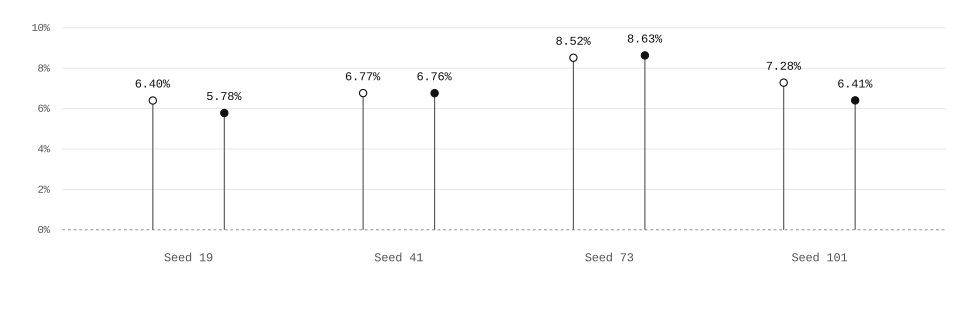
The seed numbers identify fixed randomized model fits. All four use the same market history, but their predictions can differ and therefore select different stocks. For seed 19, annualized growth is 6.40% under the baseline and 5.78% with ECQDI. For seed 73, it rises from 8.52% to 8.63%. Seed 41 is almost unchanged; seed 101 declines.
| Account | Total return | CAGR | Max drawdown | Sharpe |
|---|---|---|---|---|
| Seed 19 | ||||
| Baseline | 33.75% | 6.40% | -25.66% | 0.40 |
| With ECQDI | 30.14% | 5.78% | -26.32% | 0.37 |
| Seed 41 | ||||
| Baseline | 35.93% | 6.77% | -27.92% | 0.42 |
| With ECQDI | 35.90% | 6.76% | -27.24% | 0.42 |
| Seed 73 | ||||
| Baseline | 46.69% | 8.52% | -29.32% | 0.49 |
| With ECQDI | 47.41% | 8.63% | -27.63% | 0.50 |
| Seed 101 | ||||
| Baseline | 39.04% | 7.28% | -27.51% | 0.44 |
| With ECQDI | 33.79% | 6.41% | -26.21% | 0.40 |
Across the four accounts, mean CAGR is 7.24% for the baseline and 6.90% with ECQDI, a paired difference of -0.35 percentage points per year. This is an average of individual account growth rates, not the CAGR of a blended portfolio. The weekly implementation does not reproduce the positive average contribution seen in buy & hold.
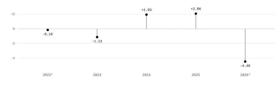
These are returns within calendar periods, averaged across seeds. They differ from grouping cohorts by their starting year. The 2022 period begins on 10 January, and 2026 ends at the 18 September price cut-off. In that latest partial period, ECQDI returns 14.12% versus 18.59% for the baseline. Recent outcomes therefore contribute to the continuous account even when the corresponding six- or twelve-month cohorts have not yet matured.
- CAGR: Annual growth rate equivalent to the account’s total return.
- Maximum drawdown: Largest peak-to-trough decline in daily account value.
- Sharpe ratio: Daily mean return / volatility, annualized over 252 sessions; no risk-free adjustment.
- Paired difference: Factor return minus the matched baseline return, under shared assumptions.
08What the evidence supports
ECQDI shows a modest historical relationship with subsequent returns and a positive average contribution to initial stock selection. Its value depends on how the score is used.
8.1 The relationship between scores and later returns
The earlier database study measures rank information coefficient, or IC: how closely the ordering of scores corresponds to the ordering of subsequent returns across calls. A positive value means higher-scoring observations tend to rank higher in later relative returns. It is neither a stock-picking hit rate nor a portfolio return.
The replay reproduces a mean monthly IC of approximately +0.032 at 63 subsequent stock bars, with a Newey-West t-statistic of 3.50 across 78 months. The Newey-West calculation allows for dependence between consecutive observations [7]. A separate timing check, excluding same-day reference calls and entering at the next available close, retains a positive 63-bar IC of +0.0321 and a t-statistic of 3.39.
View the original association estimates and their timing convention
| Forward stock bars | Mean rank IC | NW t | Months | Positive months |
|---|---|---|---|---|
| 21 | +0.0173 | 1.81 | 80 | 58.8% |
| 42 | +0.0304 | 2.93 | 79 | 64.6% |
| 63 | +0.0320 | 3.50 | 78 | 65.4% |
| 126 | +0.0408 | 3.47 | 75 | 62.7% |
This original validator enters at the third available stock close after the call. Horizons count subsequent stock bars, rather than calendar months. Monthly ICs require at least 30 calls; Newey-West lags are 1, 2, 3 and 6 months. The benchmark is the panel’s equal-weight daily return with individual daily changes clipped at ±50%. It is a research reference, not a verified investable index.
The Qlib experiment uses next-session opens, a different eligible panel and calendar-month portfolio horizons. Its returns should therefore be interpreted on their own terms. The rank association provides complementary evidence about the measurement; it does not convert directly into the paired portfolio uplift.
8.2 What remains after controlling for existing information?
Within the weekly model universe, we remove the contribution of the model’s prediction rank, prior 12-minus-1-month momentum rank and sector indicators from both score ranks and future-return ranks. The remaining rank relationship is still positive at 63 sessions. This asks whether those specified variables fully explain the association, rather than whether ECQDI is independent of every existing factor.
| Holding sessions | Raw IC | Partial IC | Partial NW t | Weeks |
|---|---|---|---|---|
| 63 | +0.0160 | +0.0214 | 2.04 | 233 |
| 126 | +0.0223 | +0.0243 | 1.65 | 219 |
Seed correlations are averaged within each date before inference. The Newey-West calculation uses 13- and 26-week lags for the two horizons. The early-period relationship is weak, and the later segment has already been inspected during research. It should not be presented as a fresh holdout for subsequent configuration choices.
8.3 Interpreting the overall result
The strongest primary interval is the twelve-month buy & hold comparison. Shorter-horizon and weekly-rebalance estimates remain consistent with no mean improvement. The continuous weekly accounts underperform on average. Taken together, the evidence supports testing ECQDI as a selective input to portfolio construction, with particular attention to decision frequency and the baseline model.
- Information timing: The next-session rule provides a buffer after same-day transcript delivery. Historical revisions require separate verification; forward records should preserve actual publication times.
- Universe coverage: Both arms share the same candidate panel. Historical membership, delisted stocks, sector assignments and adjusted-price coverage require further verification.
- Research selection: Discovery and follow-up tests reuse the same history. The single-horizon permutation and portfolio intervals do not adjust for the entire search, as explained in Appendix A.4.
- Portfolio exposures: Sector and momentum checks address specific explanations. Size, liquidity, value and other exposures need fuller controls before the contribution can be described as unexplained alpha.
- Live execution: Fixed fees and adjusted opening fills are study assumptions. Spreads, market impact, realistic order sizes and performance on newly arriving observations need separate evaluation.
The evidence is specific to the stated US panels. The originating international test did not establish replication. Further evaluation should fix the score definition and selection rules before new outcomes are known, and retain both improving and underperforming configurations in the research record.
09Verification and research access
The research records connect supplied score observations, portfolio decisions and reported results. They allow calculation checks to be distinguished from investment conclusions.
9.1 What was checked
The verification covers score replay, extraction against a saved call reference, baseline reproduction and consistency between portfolio calculations. Appendix A describes each dated run, its sample and its numerical agreement. These are internal checks against frozen inputs, rather than an external audit or a prospective performance record.
9.2 The evaluation procedure
Follow points 1-8 for each eligible weekly formation and each fixed model seed. Then summarize the paired differences, keeping policies and horizons separate.
- Load inputs. Join frozen model forecasts and eligible decision-date ECQDI scores.
- Select the baseline. Take the 50 highest-ranked eligible stocks from the model.
- Rank scores. Deprioritize the lowest 20% when at least 30 candidates have a score.
- Select with ECQDI. Take 50 stocks using the priority and tie rules in Section 4.2.
- Match assumptions. Use identical capital, allocation, prices and trading costs.
- Run both policies. Simulate buy & hold and weekly rebalance separately.
- Measure each horizon. Value completed 3-, 6- and 12-month accounts.
- Calculate the difference. Subtract the matched baseline return from the ECQDI return.
- Average seeds. Average the four paired differences within each formation.
- Summarize formations. Weight completed weeks equally and resample weekly blocks.
Continuous accounts are evaluated separately from these cohorts. Each carries its own capital through repeated decisions; its performance is not calculated by compounding the average cohort returns.
9.3 A worked stock-selection example
Table 8 shows actual candidate decisions from 10 January 2022, seed 19. Score percentiles were calculated across the full candidate set before the displayed rows were extracted. The final two columns indicate membership in the two 50-stock portfolios.
| Ticker | Model prediction | ECQDI | Lower priority | Baseline | With ECQDI |
|---|---|---|---|---|---|
| MSCI | 0.9982 | 0.0549 | Yes | Yes | No |
| TFX | 0.9163 | 0.0678 | Yes | Yes | No |
| TPR | 0.3190 | 0.4064 | No | No | Yes |
| UAL | 0.3103 | 0.7815 | No | No | Yes |
| ALB | 1.9026 | 0.7058 | No | Yes | Yes |
| DXCM | 1.4849 | 0.8398 | No | Yes | Yes |
| UA | 0.6536 | Missing | No | Yes | Yes |
A lower-priority stock can leave the baseline’s top 50 and be replaced by a candidate further down the model ranking. A missing score receives no penalty. The downloadable example includes every candidate, its source call date, score age, selection percentile and both selection decisions, so the complete ordering can be inspected.
9.4 Data for independent evaluation
The research pack includes a two-year daily ECQDI score sample in 05_additional_research_ecqdi. It uses the same dates and eligible tickers as the ECPND sample, ending eight weeks before the package release. The folder has the same five-file structure: a short README, daily scores, standalone study results, cohort comparisons and a worked selection example.
date: Decision session with score eligibility under the study’s next-session rule.ticker: Stock identifier in the eligible research universe.ecqdi_score: Value from 0 to 1; blank means no eligible value for that stock and date.
The daily file carries eligible call scores forward under the 90-calendar-day limit. It supports testing over its supplied window. Reproducing the whole 2022-2026 portfolio study also requires the earlier score history, frozen forecasts, eligibility panel and adjusted prices. Raw transcripts, the proprietary measurement and trained models are not included in the public pack.
The study files in the package contain result summaries and paired cohort returns; the example shows the full candidate-selection sequence. Return columns in the cohort CSV are decimal fractions. These records support inspection of the published averages and application rule without access to the score engine.
10Outlook and further research
The next stage is to determine where ECQDI contributes consistently: at which decisions, in which models and alongside which other information.
10.1 Configurations to carry into the next evaluation
The completed threshold tests give the score progressively more influence over selection. A 50% rule places the lower half of scored candidates in the lower-priority group; it does not require buying raw scores above 0.50. Figure 4 keeps the same score definition, baseline and 10 bp costs across the four tested settings.
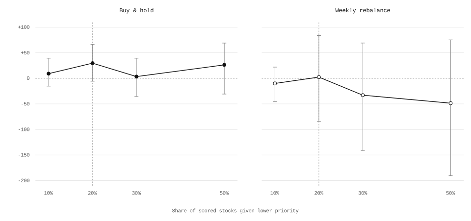
The left panel evaluates selection at entry followed by buy & hold. The right repeats selection through weekly rebalancing. Both use the full model-eligible universe, with unscored stocks remaining eligible. Each point is compared with the baseline for that policy; the common scale makes their different response to stronger selection visible.
The four buy & hold means remain positive, while the weekly mean turns negative at the stronger settings. None of these six-month intervals excludes zero. The evidence does not select a universally better threshold. Further tests should predeclare a limited set of rules and assess return, drawdown and turnover together.
- Decision frequency: Compare entry-only use with monthly and weekly decisions. The positive monthly mean is a reason to investigate slower implementation, not an established advantage.
- Score age and portfolio rules: Test shorter freshness windows, different holding periods and portfolio sizes. Keep the current 90-day limit and 20% threshold as fixed references.
- Coverage and exposures: Compare the full and scored-only universes, retain matched baselines and extend controls for sector, size, momentum, liquidity and volatility.
- Other models: Apply a small set of declared rules to independently chosen rankings. Separate changes to the portfolio application from changes to the text-score definition.
10.2 Prospective evaluation
A forward ECQDI test should record each score before its subsequent return is known. It should fix the measurement version, eligible universe, score-age rule and portfolio configuration in advance, and preserve the actual observation and publication times. Later corrections should create new records while leaving the original decision snapshot inspectable.
Matched baseline and ECQDI accounts can then record selections, trades, costs and daily values as new data arrive. Missed decisions should remain documented rather than filled retrospectively. Three-, six- and twelve-month cohorts should enter horizon summaries only after completion. A broker paper account, if used, should retain its fills separately from the internal simulation and from real-money results.
This note reports historical ECQDI evidence. It does not present a verified ECQDI forward track record or establish that the live ECPND service already delivers this second factor. A prospective ECQDI evaluation needs its own start date, protocol and maturity counts.
10.3 Combining quantitative questioning with participation history
ECPND - Earnings Call Participation Network and Dynamics examines who participates and the eligible history connecting those participants across companies. ECQDI adds a text-based view of quantitative questioning. Their mean cross-sectional rank correlation is +0.076 in the combined study: they frequently order stocks differently, providing a concrete reason to examine complementary use.
The combined-factor paper compares the price model, each factor alone and joint selection rules on the same forecasts and prices. Its initial 50/50 combination averages the factors’ current percentile ranks before applying a 20% lower-priority threshold. A missing component receives a neutral rank of 0.5; two missing components produce no penalty.
View the initial single-factor and combined comparisons
| Selection | 6M B&H return | Mean weekly CAGR |
|---|---|---|
| Qlib baseline | 6.05% | 7.24% |
| With ECPND | 6.59% | 8.33% |
| With ECQDI | 6.34% | 6.90% |
| Both · 50/50 ranks | 6.43% | 7.85% |
| Both · simultaneous filters | 6.78% | 7.55% |
These are results from a separate matched experiment. The six-month column reports buy & hold returns; the annualized column reports mean growth across continuous weekly accounts.
The equal-rank combination improves on the price baseline but trails ECPND alone in mean continuous CAGR: 7.85% versus 8.33%. An alternative rule that deprioritizes a stock when either score falls in its lowest fifth raises six-month buy & hold uplift to approximately +74 bp versus Qlib. However, it trails an equally restrictive ECPND-only control by 11.2 bp. A broader filter and a more informative second input are different explanations for an improved result.
The weight-and-threshold extension evaluates 60 rules and 52 controls matched to the number of lower-priority candidates. One example, 75% ECPND and 25% ECQDI rank weight at the 20% threshold, adds about +69 bp versus Qlib over six months, compared with +54 bp for ECPND alone. Its incremental interval versus ECPND includes zero, and its later-period advantage narrows to 2.2 bp. The weights apply to score ranks, not portfolio capital.
The next combined test should retain all four references: the unchanged price model, ECPND alone, ECQDI alone and a fixed combination. Low correlation is useful motivation, but value comes from improving a matched portfolio after costs and exposure controls. The individual uplifts cannot simply be added.
Research status. Configuration and combination tests reuse previously studied history. Their intervals describe individual comparisons and do not correct for selecting among all tested alternatives. The primary ECQDI results in this note remain based on the 20% rule; future versions and forward tests should be reported separately.
-References
- Mayew, W. J., Sharp, N. Y. & Venkatachalam, M. (2013). Using earnings conference calls to identify analysts with superior private information. Review of Accounting Studies, 18(2), 386-413. doi:10.1007/s11142-012-9210-y.
- Rennekamp, K. M., Sethuraman, M. & Steenhoven, B. A. (2022). Engagement in earnings conference calls. Journal of Accounting and Economics, 74(1), 101498. doi:10.1016/j.jacceco.2022.101498.
- Yang, X., Liu, W., Zhou, D., Bian, J. & Liu, T.-Y. (2020). Qlib: An AI-oriented Quantitative Investment Platform. arXiv:2009.11189. Official Microsoft repository.
- Microsoft Qlib. Alpha158 data handler. Official implementation and feature-processing interface. Accessed 25 September 2026. The study uses 157 available features from this family.
- Ke, G., Meng, Q., Finley, T., Wang, T., Chen, W., Ma, W., Ye, Q. & Liu, T.-Y. (2017). LightGBM: A Highly Efficient Gradient Boosting Decision Tree. Advances in Neural Information Processing Systems 30.
- Politis, D. N. & Romano, J. P. (1991). A Circular Block-Resampling Procedure for Stationary Data. Stanford Department of Statistics, technical report EFS NSF 370. The block lengths and resampling counts are this study’s implementation choices.
- Newey, W. K. & West, K. D. (1987). A Simple, Positive Semi-Definite, Heteroskedasticity and Autocorrelation Consistent Covariance Matrix. Econometrica, 55(3), 703-708. NBER working-paper version.
AAppendix: Study evidence and verification
This appendix records the score replay, the long-only portfolio comparison and the follow-up checks behind this edition. It separates reproduction of an earlier calculation from evidence about its investment usefulness.
A.1 Extraction and score replay - 24 September 2026
The recovered ECQDI snapshot contains 78,851 calls and 48,701 stored version-2 scores. Replaying the stored score definition reproduces all 48,701 values exactly. A separate extraction check matches the saved reference for 630 calls. These checks establish agreement with the recorded implementation and reference data; they do not establish future return predictability.
The portfolio study applies a stricter historical ordering rule: the sector reference contains only calls from earlier dates. It excludes other calls held on the observation’s own date, regardless of their processing order. Under this convention, 48,689 call scores remain eligible. Reversing the order of same-day records leaves the strict-date calculation unchanged. The daily portfolio join then accepts only prior-call observations whose age does not exceed 90 calendar days.
A.2 Long-only Qlib comparison - 24 September 2026
The primary run combines those scores with the frozen Qlib forecasts and adjusted prices, through 18 September 2026. It evaluates both arms under buy & hold and weekly rebalancing for four model seeds. The 232 formations with at least one completed horizon produce 3,712 account paths. A path can supply three-, six- and twelve-month outcomes as those horizons mature.
No incomplete portfolio scenarios are recorded. All six baseline horizon means and all four continuous baseline accounts agree with their earlier recorded results within 3 × 10-15 in return units. Twenty year/seed training records satisfy the chronology checks, and no model forecast is dated on or after its execution. These are checks of model and portfolio timing; transcript publication and revision records are a separate source-data question.
Figures 1-3 and Tables 1, 2 and 5 draw on the reviewed source, primary portfolio and calendar-account records. The tiny reproduction differences reflect numerical agreement between calculations, rather than that level of precision in expected returns.
A.3 Selection, cost and attribution checks - 24 September 2026
The follow-up holds the underlying score definition and forecast history fixed while examining thresholds, scored-only eligibility, sector matching, costs and rebalancing frequency. It records 27,840 cohort account scenarios with no data gaps. These simulations reuse the same historical observations; their count describes computational scope rather than independent evidence.
The primary results are reproduced before the extended comparisons are interpreted, with a maximum difference below 3 × 10-16. A separate accounting comparison checks returns, drawdowns, turnover and stock contributions against the reference simulator at two formation dates for seed 19, across both arms and portfolio policies. Its 4,787 scalar comparisons have a maximum absolute discrepancy below 4 × 10-13. This is an internal consistency check of the sampled calculations.
Tables 3-4 and Figure 4 use these follow-up results. Table 7 reports the conditional rank-association checks, while Table 8 extracts actual candidate decisions from the first primary formation. The combination aggregates in Table 9 come from the separate experiment dated 25 September 2026; the wider weighting study is documented in the combined-factor note.
A.4 Discovery checks and corrections to the earlier study
The originating search examined 131 features at four horizons, or 524 combinations. A replicated permutation check shuffles returns within months and repeats the qualifying-feature search at the 63-bar horizon. Thirteen of 300 shuffled maxima reach the observed statistic. The original fraction is 0.0433; including the observed sample under the finite-simulation plus-one convention gives 0.0465.
This procedure tests selection among features at that horizon. It does not repeat the maximum across all four horizons or every previous research branch. Eight features meet the implemented 63-bar qualification conditions; ECQDI’s measurement is the highest qualifying result, rather than the only one. No test survives the original 10% Benjamini-Hochberg procedure over all 524 combinations. These procedures answer different questions, so the single-horizon permutation is not a correction for the whole research history.
The earlier standalone long/short study also required correction. It used current-month thresholds for trades earlier in the month and incomplete capital and turnover accounting. A corrected funded account uses prior-month thresholds, next-session-close entry, daily cash and share accounting, and borrowing charges. It produces 1.20% CAGR at 10 bp execution costs with an illustrative 2% annual borrow rate, and -1.94% at 20 bp. These belong to a separate long/short experiment and are not the long-only uplift in this note.
The originating technical-model blend and its placebo result are likewise not transferred to this Qlib comparison. Table 6 retains the original association validator’s third-close entry, while the main portfolio study uses next-session opens. Keeping the protocols distinct prevents a successful check under one design from being presented as validation of another.
A.5 Published records and evidence versions
The study downloads provide primary results, paired cohort returns and candidate decisions. The research pack adds the delayed two-year daily score sample described in Section 9. Together they support inspection of the reported averages and independent score evaluation, without publishing the proprietary text measurement.
Tables and charts are generated from the reviewed evidence snapshot, which records the hashes of its underlying reports and public-data inputs. The study-results JSON includes the snapshot digest. Matching SHA-256 values identify identical file contents and distinguish this edition from a later recomputation; they identify evidence versions rather than certify an investment result.
Evidence versions and SHA-256 checksums
Reviewed ECQDI evidence - 25 September 20267a0d9091d96b98e8a5b49e01cb3447d55fbf3de76af1c6263865e0d3bc121f09
Primary long-only comparison - 24 September 2026be6f089918d79e6a4cdc0594edaa4ef3d2fb255f959a902d36057a3c280f2d83
Selection, cost and attribution follow-up - 24 September 20267552863cb8cb7b2f3f31ec4bd14dc4cd12fd6d0f4a3f8f23388e2a4d3ca3d644
Extraction reference verification - 24 September 202667a9bb5f16b7483a03f34afcfaf4419595cdd927804241dd1a2b657bfca41716